Radio Communications

Radio control panel

The main development goal for this year (2019) is to have fully operational space stations to dock to. Yet after the work on the collision physics an issue quickly appeared about the docking ports: where should the related information be stored and how to pass it to the ship’s flight controller?

On a monday morning in July I decided not to duplicate the data and have the stations broadcast the necessary information through a radio link: should have been a 3 hour quick-and-dirty hack… But as it turned out it actually became a 3 month implementation of a full new game system! 馃榾

It’s not actually a delay since I’m planning to spend a lot of time on the ship’s sensors and electronic warfare equipment starting next year. So it’s rather an “unexpected optimization of the project’s work items” 馃檪

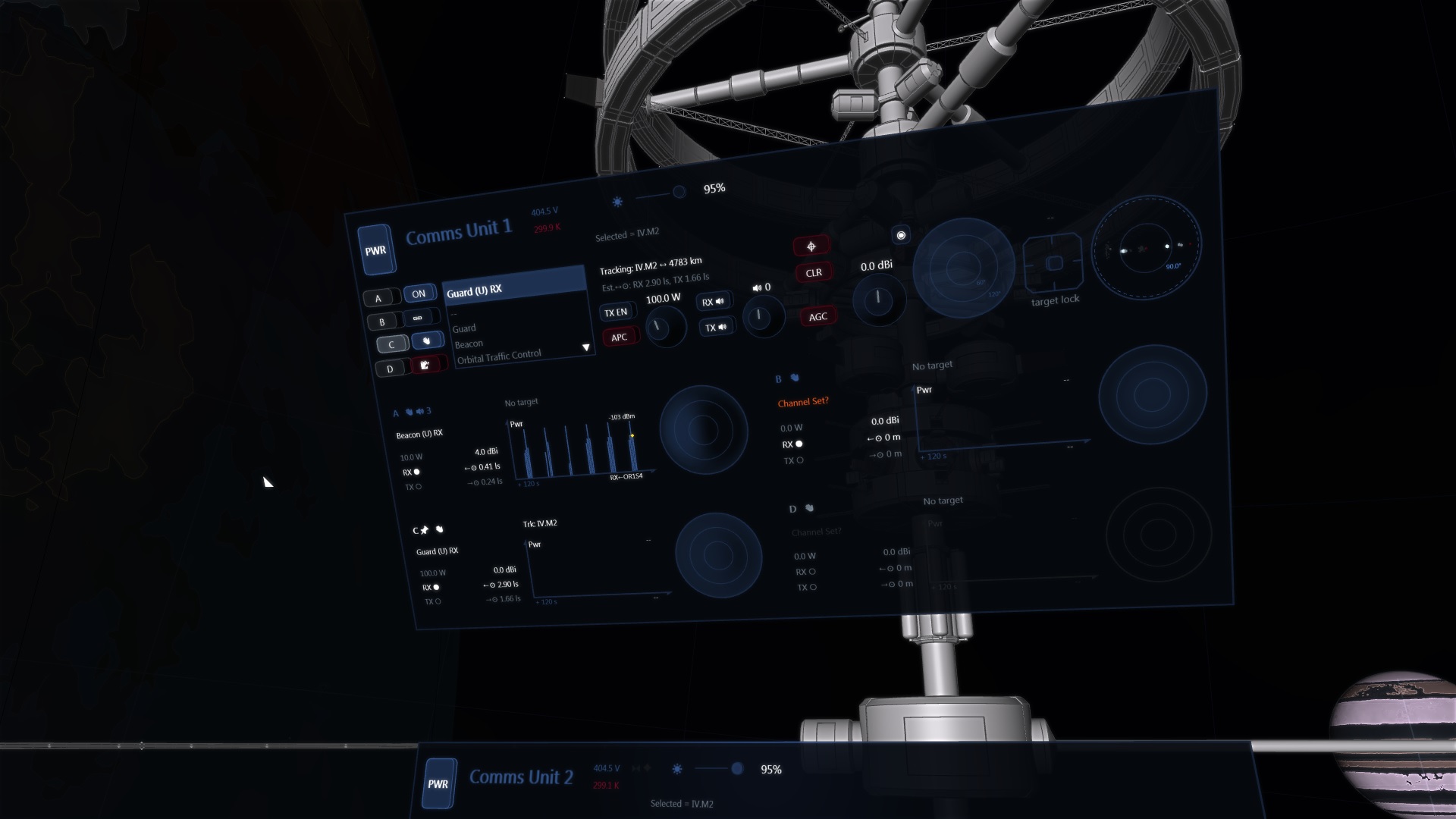
Like with the other systems the model attempts to be as realistic as possible while hopefully offering interesting gameplay elements:

  • allocation and configuration of the radio resources,
  • search for contacts (in space and across the different channel sets),
  • management of trade-offs between coverage of nearby surroundings and effective range…

Having to use the on-board systems to sense the ship’s environment and actively search for contacts and information is very dear to me. IMHO it’s really a pity when games dumb down this part and directly display some green and red dots on a “radar display”. To me that’s really missing the “hunting” fun.

Typical operations of the ship’s comms units are presented in the following video:

The underlying model is presented here.

Technically the travelling packets are kept alive as long as they may be received. An interesting twist with modelling a proper propagation velocity (speed of light) is that a radio device might be configured for a successful reception long after the message was emitted!

Also since this is not a frame critical system most of the workload is managed in parallel on a worker thread. It’s largely overkill at the moment but a stellar system might contain many communicating devices in the future. Also I’m planning to reuse the infrastructure to model the ship’s radars and jammers.

Thanks for reading!

Leave a Reply

Radio Communications

Radio Link Analysis

Radio communication systems use electromagnetic waves to carry out information from a transmitter to a receiver.

  • The transmitter side is commonly labeled TX,
  • and the receiver’s RX.

Information is energy and messages are broadcasted at a set power PTX [W] (watts). Evaluating a radio transmission then requires to answer two questions:

  1. Determine PRX = the fraction of PTX that effectively reaches the receiver.
  2. Check whether PRX is large enough for the message to be intelligible.

Signal Propagation and Antennas

Isotropic emission

A TX source that is radiating power equally in all directions is called “isotropic” (think of a light bulb). The wavefront is thus a sphere expanding at the speed of light (“c”).
When it reaches the receiver at a distance “d” its power is spread over the corresponding sphere area = 4蟺d虏. That is its power density per unit area equals PTX / 4蟺d虏 [W/m虏].
The receiver’s antenna is characterized by its effective area Aeff or “aperture”聽 [m虏] as seen from the source (ex: the dish of a parabolic antenna). The received signal’s power is then Aeff * TX power density at distance d.

Focused Beam: Antenna Gain


Radio emissions can also be focused into a beam (similarly as a flashlight). This聽 is called “directivity“. The TX power density is larger inside the beam since the power is spread over a smaller portion of space. This effect is characterized by the Antenna Gain GTX, which measures the resulting amplification with respect to an ideal isotropic source.
ex: in the case of the cone shown above, GTX = 2 / (1 – cos 胃/2), with 胃 the cone’s apex angle.

The antenna gain is generally expressed in decibels (the logarithmic scale is convenient for widely varying values), with a dBi unit where “i” refers to the ratio to an ideal isotropic source.
GTXdB = 10路log10(GTX) [dBi]

RX Antenna Gain

In a reciprocal way to what happens in TX, the receiving antenna can also be directive. That is its effective area Aeff is oriented and varies depending on the direction of the incident wave.
The corresponding gain is similarly defined as the ratio of the effective aperture to the area of an ideal isotropic antenna:

where 位 is the wavelength of the signal.

PRX may thus be also expressed as:However depending on the type of antenna in use this may hide the more physical effective area quantity Aeff. (ex: for a parabolic antenna Aeff is directly proportional to the dish area).

Radiation Pattern

The gain of directive antennas is maximum along the beam’s direction as defined above. That is its actual value depends on the relative angle between the TX鈫扲X line and the beam’s direction. The corresponding function G(<TX鈫扲X, beam>) is called the antenna’s “radiation pattern“.
Real radiation patterns can be very complex and generally feature multiple lobes. However ASG supposes smart active antennas with a single main beam (+ some isotropic leakage). Typical patterns corresponding to various gain settings are shown below. The beam is in the “0掳” direction, the plot provides the gain value at the given angle (in linear scale):

Note: the 1.7 dBi configuration is typically used by space stations with their parent body at 180掳. This provides a slightly larger range towards outer orbits while maintaining a full coverage.

Polarization” relates to the orientation of the electric field in radio waves and can further reduce the power collected by a receiver. For simplicity the game models an average 2 dB mismatch penalty on all transmissions.

Receiver Sensitivity

Bit Rate and Signal to Noise Ratio (SNR)

Digital communications transmit information exactly as a language does: a message is a sentence composed of words called “symbols“. The conversion process of a message into actual radio waves is called “modulation“.

Obviously shorter symbol times = higher symbol rates carry more data in a given amount of time. Moreover the richer the vocabulary (= the number of different symbols in use) the more the information carried by each symbol.

Information is measured in bits. A bit can take 2 values so for instance a symbol that can be represented as a dot in a 4 x 4 grid carries 2 + 2 = 4 bits.

In combination with the symbol rate this simply yields: Bit Rate = Symbol Rate x Bits per symbol.

However it appears very clearly that when symbols can take many values it becomes more and more difficult to distinguish between them. Using the language metaphor again this is like different but similar sounding words ex: “lose” and “loose”.

Furthermore communication systems are not perfect and subject to perturbations of various natures. These are commonly referred to as “noise” and produce some uncertainty in the received symbols (the fuzzy, larger dots on the figure to the left).

聽The Signal to Noise Ratio measures the ratio of the signal power to the noise power:Naturally, the more complex a modulation (more bits per symbol), the less its immunity to noise and the larger the required SNRdemod for error-free transmissions (here “demod” refers to a successful demodulation at the receiver).

Channel Bandwidth and Antenna Noise

These two quantities are linked because together they let us estimate the noise power at the receiver as explained below.

The channel bandwidth designates the range “B” [Hz] of the electromagnetic spectrum that is occupied by a transmission signal. It depends on the actual waveforms but is directly proportional to the symbol rate.

The main source of the perturbations mentioned above聽 is the the thermal noise from the antenna itself. It is due to the random motion of the electrons and is called a “white noise” because it exhibits a constant power density across the entire spectrum:
P[W/Hz] = kB路T where kB is Boltzmann’s constant [J/K] and T is the absolute temperature [K].

Finally to select the wanted signal within the entire spectrum the receiver applies a bandpass filter with bandwidth = “B” (to avoid degrading the transmitted information while filtering out as much unwanted neighboring power as possible). However since the antenna noise is constant over the whole band with density kB路T [W/Hz], the noise power at the receiver input is
PN,RX = kB路T路B [W].

Sensitivity

The main quantities to compute the minimum RX power for a successful transmission are now available:

  • given the channel bandwidth B,
  • the noise power is kB路T路B,
  • and the signal power for a successful demodulation is kB路T路B路SNRdemod

The last major contribution is the receiver itself. The quantity kB路T路B路SNRdemod is usually very small and requires a large amplification so that it can be processed. The related active circuit adds some noise itself and slightly degrades the effective SNR. This requires to further increase the signal power by the receiver’s “noise factor F“. Finally:

The bandwidth and SNR terms explain why the range of high bit-rate communications is usually quite limited: their symbol rate requires a large channel bandwidth and the complexity of their modulation a strong SNR.

In order to make the transmitted data more resilient to noise, communication systems use various techniques on top of the modulation itself. This can include some amount of repetition, grouping the data to minimize the risk of misunderstanding, or providing some “context” at the whole message level to help reconstruct meaningful sentences.
However this means that there is a loss of effective data bit rate as the correction information must be passed along with the initial message.

CSN F9 Comms Units

The ship is fitted with 3 distinct devices, each with its independent hardware and 4 software slots. This provides both redundancy and the ability to maintain numerous simultaneous radio links with many purposes:

  • Orbital Traffic Control,
  • Space Positioning System (high-precision navigation in the equipped areas),
  • Traffic monitoring (beacons, emergency calls…) and related comms,
  • Interstellar Data Network (“the mail” to carry the latest information during interstellar trips),
  • Control and Data Links with tactical assets,
  • Detection and Surveillance,

Phased Arrays

Each unit features 2 phased arrays. These are complex active systems built from a network of unit antennas that are coordinated to produce some desired global characteristics. In effect they provide the ability to:

  • control the shape of the overall radiation pattern and form a beam with tunable gain,
  • steer the beam in any direction around the ship.

Adjusting the gain provides the ability to search for trade-offs between range and space coverage. At maximum gain an array will arrange its elements to offer the maximum effective area in the selected direction. At lower settings it reorganizes them to maximize the effective area over the whole arc.

The arrays are mounted on the hull at mid-ship. They provide a coverage with axial symmetry but with a larger effective area at right angle from the ship’s axis.聽 In this plane the formed beams will allow for higher gains and larger ranges. It might thus be useful to steer the ship to optimize the radio equipment performance in some circumstances.

The 2 arrays correspond to 2 broad frequency bands:

  • UHF (‘U’ for ‘Ultra’ high frequencies, around 1 GHz) for all general communications,
  • SHF (‘S’ for ‘Super’ high frequencies, around 10 GHz) for directional point-to-point links,

Indeed for a given effective area, the higher the frequency the smaller the wavelength and the larger the gain. As a result the SHF array is mainly used for point-to-point communications. The choice of the UHF band is a trade-off taking into account effective ranges, space coverage and immunity to the parasitic emissions from fusion reactors.

Channel Sets

“Channel Sets” encompass a set of technical characteristics that define the underlying radio link, and are generally associated to a specific purpose (exactly as “WiFi” is used to build local data networks, or “4G” represents cellular comms).

Once a channel set has been selected the comms unit automatically handles the low-level technical configuration (specific channel frequencies, synchronization, signaling protocols…). Note that multiple links to different devices can be maintained by a single slot over the same set (again exactly as multiple devices can connect to a WiFi network).

The following table lists the defined sets:

Control Panel

The figure below presents an annotated view of a comms unit control panel:

Comms Unit control panel - sensors station

Typical usage is demonstrated in the following video: