Integrated flight planner

Celestial navigation is a very difficult task. All involved objects are in continuous motion and gravity alone makes their trajectories (conic sections) far from straightforward. Also describing the state of a simple mobile requires no fewer than 7 variables:
time, position (x, y, z) and velocity (vx, vy, vz) using Cartesian coordinates for instance.
The problem is also inherently “chaotic” in the mathematical sense, that is extremely sensitive to the initial conditions (butterfly effect). A small loss of accuracy can easily escalate into a complete failure to reach a destination.

Nevertheless this should not prevent you from performing your mission and the CSN F9 features an advanced suite of flight planning tools to let you find your way. It is organized around a core map and  three flight planning modes presented in the sections below:

to the left: automatic flight planner panel

4D celestial map

The navigator’s station is fundamentally a map. However it is not a static one (nor is it slaved to real time) because a static (or near static) 3D view would be a truncated representation while all objects are constantly moving. Instead the primary characteristic of the display is that time can be freely swept forward and backward. This way you can properly visualize the dynamics of the problem and why the “4D” label i.e. 3 dimensions of space + time.

Incidentally the ship’s planned trajectory establishes a 1 to 1 correspondence between space and time: along its flight path the ship is one specific place at one specific time. The trajectory cursor (red dot) symbolizes this relationship:

  • you can adjust the time variable and have the cursor placed accordingly
  • the other way around placing it on the path will change the time to match the chosen location

Now switching from time to space. All massive celestial bodies generate a gravity field and with it a region within which their attractive force has a dominant effect on all present objects. This region is called their Sphere of Influence (“SOI”) and in your ship’s navigation software space is in effect partitioned into a tree of nested SOIs with the galaxy at its root.
Also the trajectory is generally split into multiple legs and each one of them is displayed in its parent’s SOI. This is to easily understand the nature of the motion: a stable elliptic orbit around a moon appears as a complex helix as seen from its parent planet’s reference frame. The continuity of the trajectory across SOI boundaries appears clearly when sweeping time.

The map time control function is demonstrated in the following video :

Trajectory propagator and manual planning

The trajectory propagator is the heart of the flight planning routines. Its role is to derive the trajectory and vessel state over time (mass) resulting from a given set of maneuvers, initial conditions and a ship and propulsion model.

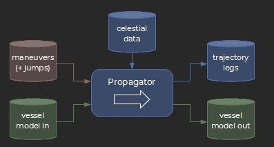
The path legs are computed using two methods:
→ as a conic section when submitted to a single central gravity force
→ through numerical integration in all other cases (i.e. with multiple acting forces), including when the ship is maneuvering, in an atmosphere or close to a star barycenter (3-body model).

A new leg is started at each change of the propagation conditions: starting or stopping the engine, crossing a SOI boundary etc…

Note: the CSN F9’s navigation software treats all maneuvers as “finite” (i.e. not “impulsive” or instantaneous) and the motion is numerically integrated while thrust is applied. Even in average gravity wells the traveled distance during burns remains significant and neglecting it would lead to unacceptable errors, especially considering that the margin of error for a successful jump is less than 100 m. Furthermore the flight controller uses the computed path as a guidance reference to keep the ship on track during burns.

In direct connection with the trajectory propagator the most basic flight planning method is then to manually insert maneuvers and adjust their parameters. The flight plan editor provides the necessary controls together with the data needed to aim at a chosen target. This is demonstrated in the video below:

Semi-automatic flight planning routines

To spare you the tedious work of manually tuning all maneuvers, the flight planner features some specific routines to automatically manage the most common navigation tasks:

  • transfer to a target (with optional rendezvous)
  • circularization
  • course correction to a jump-point (and jump insertion)

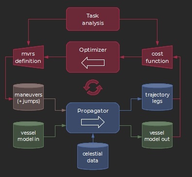
These routines elaborate on the forward propagation model by closing the loop through a numerical optimizer. Typically a maneuver is inserted and its parameters automatically tuned so as to meet the task’s objectives.
The process is iterative and similar in essence to the manual method when trying to achieve some specific results. Besides the automation the main difference is a better management of multivariate searches (gradient based instead of variable per variable).

The “transfer to target” routine is shown in the following video:

Automatic flight planner

Manual and assisted methods may be enough for simple maneuvers and short trips. However long distance flights are much more difficult to plan because of the staggering number of possible transfer and jump options along the way. Manually building and tuning many paths to finally pick the most efficient one is just plain impractical.

To cope with the problem your navigation suite features an automatic path finder and router:
give it a destination and it will compute a set of maneuvers and jumps to efficiently get there.

The process is essentially run in two steps:

  1. it starts with a search through the graph of all possible paths based on heuristic functions to estimate the travel time and minimize the overall ΔV cost,
  2. once a path has been picked the semi-automatic forward planning routines previously described are used to build the trajectory. In case of a non-solvable routing problem the algorithm may retry with a slightly different path (with a limited number of attempts).

Tuning parameters

NB: clicking a parameter’s name resets its value to default.

Eco, Nom, and Max thrust [kN]
By default the algorithm will try to use the “economical” (= lowest) thrust setting for maneuvers, then will revert to nominal or maximum thrust when facing routing difficulties. You can adjust these inputs to suit specific needs and your ship’s performance (especially after upgrades)

Safety level [hours]
This characterizes the required minimum collision-free coasting time at a jump exit. A jump solution is not considered safe (and thus discarded) if – without any maneuvering – a collision occurs before the set limit. You might want to toughen the requirement if your ship is in bad condition (in anticipation of possible mechanical problems), or on the contrary lessen the value to help find a solution on complex trips. The log window indicates when a reset is triggered by failed safety conditions. The default is 1 hour.

Per jump penalty [km/s]
The higher the value the more costly jumps appear to the algorithm. This is added to the actual cost estimation. The default is 20 km/s.

Flight time multiplier
The total flight time to a destination is impossible to predict beforehand since it depends on the chosen solution. As a result the algorithm heuristically derives a nominal time schedule as it is running though the graph of possible paths. The “flight time multiplier” is simply a global multiplier on all the internal time estimations and so you can use it to factor in your mission-related constraints. In general allowing more time reduces the ΔV cost. On the other hand while reviewing the trajectory you may notice situations where the ship remains parked on a waiting orbit before a jump, this is typically a hint that the time constraint may be easily toughened.

The video below demonstrates the use of the automatic flight planner.

What to do when no solution can be found?

Obviously with a ΔV budget around 100 km/s the ship cannot cross the galaxy on a single run, and longer trips may require refueling stops (additional tools are in the work to help with the related “strategic navigation” planning).

Also some locations just cannot be reached, for instance dwarf planets that might not be massive enough to harbor galactic jump-points and still weight too much for in-system connections. Other objects may only get within reach at certain times: this is typically the case of interior terrestrial planets with large orbital velocities.
On the other hand such locations are unlikely to be target destinations for your missions. In any case you will always be given the opportunity to carefully study a potential assignment before committing to it.

Furthermore as previously mentioned the simultaneous motion of all celestial bodies makes the problem highly dynamic, and consequently it is often interesting to try a sensitivity analysis and check the effects of small adjustments of the input parameters (critical jump ΔV and time multiplier primarily), especially on complex multi-jump trips.

How-to: station to station flight planning video